
A Complete Introduction To Time Series Analysis (with R):: Classical Decomposition Model part II
In the last article, we introduced the classical decomposition model, and had a comprehensive discussion of trend estimation, notably using the moving average filter. This time, we will discuss the final missing part: seasonality.
Estimating Seasonality
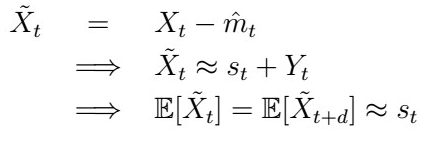
Assume that Yt is some White Noise process, and consider the classical decomposition model
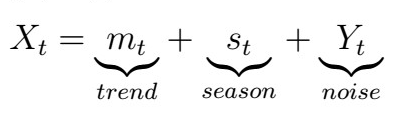
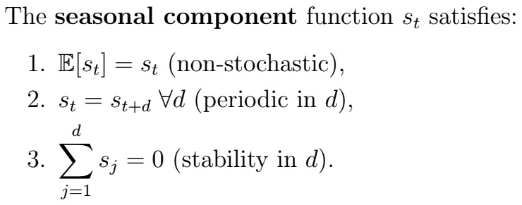
The equations above are just mathematical formalizations of the notion that the process “kind of behaves similarly” every certain period or season. For instance, you can expect winter to start roughly at the same time every year (even in Canada, where we have winter 8 months a year). How can we estimate this seasonal component? Suppose we have some series
Suppose also, that these data have some seasonal function with a period d. We let k=1,..,d be an index ranging over each season. In order to estimate the seasonal component, we follow the next procedure:

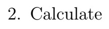
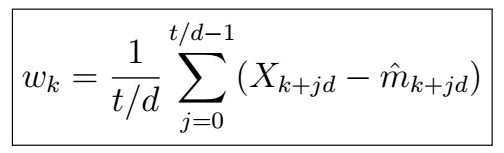


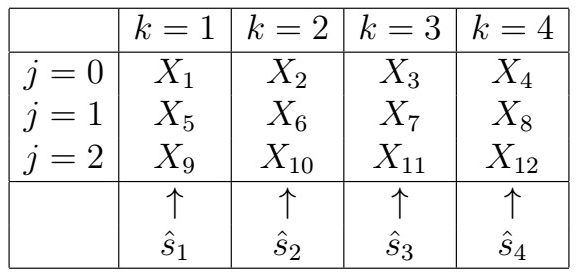
The following table might be helpful for visualization for 12 observations and four seasons:
Classical Decomposition Analysis
Now that we are equipped with the tools to estimate seasonality, let’s jump right to the classical decomposition analysis , that is, the procedure to follow to analyze any time series, assuming a classical decomposition.

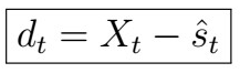
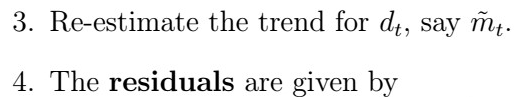
2. Estimate the seasonal component using the procedure presented before, and obtain deseasonalized data dt.
Hopefully, the resulting Yt-tilde should look like white noise, which tells us that our analysis was correct. Let’s see a full-worked example!
How to R
First, load all the required libraries:
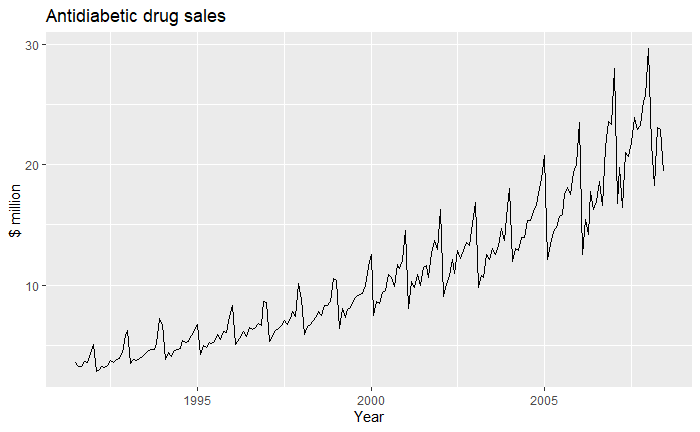
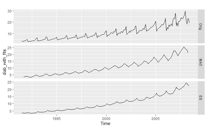
In this example, we consider the anti-diabetic drugs sale data, which can be found in the package fpp2 :
It is clear that not only there is a trend, but also some seasonal component that repeats every year, when the sales suddenly spike. We can estimate the trend with the ma function (that is, we are fitting a moving-average) and also the ses function, for exponential smoothing with alpha=0.2.
We see that these average estimates also capture some of the seasonality. How do we know which one is better? We can inspect the residuals:
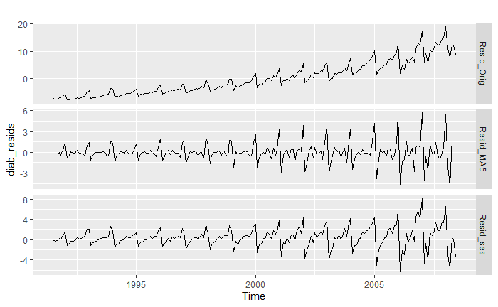
We see from the residuals that the exponential smoothing was perhaps a bit too much of an overkill, and overall the MA5 residuals look closer to White Noise. Now, our task is to estimate seasonality: for this sake, we will obtain the frequency of the data observations (that is, the number of seasons), and plot what this seasonality looks like:
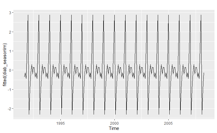
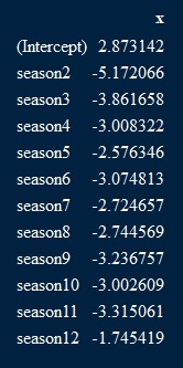
We see that indeed the peaks are exactly every 12 seasons (that is, every 12 months= a year). We can even obtain the coefficients for this model:
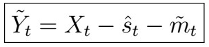
Next, we remove this seasonal component, and hope that the result looks somehow like a White Noise process:
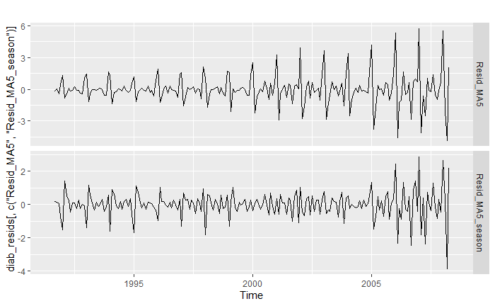
The second graph here shows the residuals after removing the seasonal component. Don’t be fooled by the shape! Note that the range goes (mostly) from -2.5 to 2, as opposed to -3.5 to almost 6 in the MA5 residuals. Except for the last couple of years, it looks like the process is closer to White Noise. Let’s inspect the ACF plots:
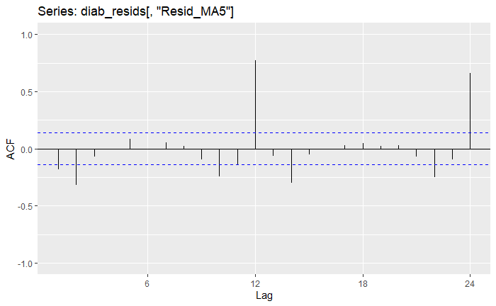
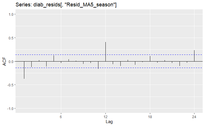
The residual definitely look better for the detrended and deseasonalized series. For the sake of illustration and as a summary, we can compare the original data against the deseasonalized data only, as well as the detrended and deseasonalized data residuals:
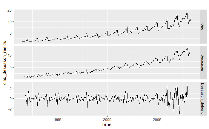
That’s quite some progress! You might still be wondering “that’s awesome, but why are we doing this?”. We will answer that question in-depth much later, but the spoiler is the following: if we can obtain good, approximately White Noise residuals, we can fit better models, and then simply add back the trend and seasonal components at prediction time :)
Next time
That was a lot! If you have been following these article series, by now you should feel comfortable with performing full classical analysis on any time series on your own. In the next article, we will learn about another tool that will help us better analyze trend and seasonality: differencing. Stay tuned, and happy learning!


